options(stringsAsFactors = FALSE)
library(tm)

textdata <- read.csv("data/sotu.csv", sep = ";", encoding = "UTF-8")
english_stopwords <- readLines("resources/stopwords_en.txt", encoding = "UTF-8")

# Create corpus object
m <- list(ID = "id", content = "text", DateTimeStamp = "date")
myReader <- readTabular(mapping = m)
corpus <- Corpus(DataframeSource(textdata), readerControl = list(reader = myReader))

1 Sentence detection

The separation of the text into semantic analysis units is important for co-occurrence analysis. Context windows can be for instance documents, paragraphs or sentences or neighbouring words. One of the most frequently used context window is the sentence.

Documents are decomposed into sentences. Senteces are defined as a separate (quasi-)documents in a new corpus object of the tm-package. The further application of the tm-package functions remains the same. In contrast to previous exercises, however, we now use sentences which are stored as individual documents in the body.

Important: The sentence segmentation must take place before the other preprocessing steps because the sentence-segmentation-model relies on intact word forms and punctuation marks.

The following code defines two functions. One selects documents, the other decomposes a given document text into sentences with the help of a probabilistic model.

require(openNLP)

# Function to convert a document in a vector of sentences
convert_text_to_sentences <- function(text, lang = "en", SentModel = "resources/en-sent.bin") {
  
  # Calculate sentenve boundaries as annotation with Apache OpenNLP Maxent-sentence-detector.
  sentence_token_annotator <- Maxent_Sent_Token_Annotator(language = lang, model = SentModel)
  
  # Convert text to NLP string
  text <- NLP::as.String(text)
  
  # Annotate the sentence boundaries
  sentenceBoundaries <- NLP::annotate(text, sentence_token_annotator)
  
  # Select sentences as rows of a new matrix
  sentences <- text[sentenceBoundaries]
  
  # return the sentences
  return(sentences)
}

# Function to convert a corpus of documents into a corpus of single sentences from documents
reshape_corpus <- function(currentCorpus, ...) {
  
  # Extraction of all sentences from the corpus as a list
  text <- lapply(currentCorpus, as.character)
  
  # convert the text
  pb <- txtProgressBar(min=0, max=length(text))
  i <- 0
  docs <- lapply(text, FUN=function(x){
    i <<- i + 1
    setTxtProgressBar(pb, i)
    convert_text_to_sentences(x)
  }, ...)
  close(pb)
  
  docs <- as.vector(unlist(docs))
  
  # Create a new corpus of the segmented sentences
  newCorpus <- Corpus(VectorSource(docs))
  
  return(newCorpus)
}

We apply the function reshape_corpus on our corpus of full speeches to receive a corpus of sentences.

# original corpus length and its first document
length(corpus)

## [1] 231

substr(as.character(corpus[[1]]), 0, 200)

## [1] "Fellow-Citizens of the Senate and House of Representatives:\n\nI embrace with great satisfaction the opportunity which now presents itself\nof congratulating you on the present favorable prospects of our"

# reshape into sentences
sentenceCorpus <- reshape_corpus(corpus)

## ===========================================================================

# reshaped corpus length and its first 'document'
length(sentenceCorpus)

## [1] 62517

as.character(sentenceCorpus[[1]])

## [1] "Fellow-Citizens of the Senate and House of Representatives:\n\nI embrace with great satisfaction the opportunity which now presents itself\nof congratulating you on the present favorable prospects of our public\naffairs."

as.character(sentenceCorpus[[2]])

## [1] "The recent accession of the important state of North Carolina to\nthe Constitution of the United States (of which official information has\nbeen received), the rising credit and respectability of our country, the\ngeneral and increasing good will toward the government of the Union, and\nthe concord, peace, and plenty with which we are blessed are circumstances\nauspicious in an eminent degree to our national prosperity."

CAUTION: The newly decomposed corpus has now reached a considerable size of 62517 sentences. Older computers may get in trouble because of insufficient memory during this preprocessing step.

Now we are returning to our usual pre-processing chain and apply it on the separated sentences.

# Preprocessing chain
sentenceCorpus <- tm_map(sentenceCorpus, removePunctuation, preserve_intra_word_dashes = TRUE)
sentenceCorpus <- tm_map(sentenceCorpus, removeNumbers)
sentenceCorpus <- tm_map(sentenceCorpus, content_transformer(tolower))
sentenceCorpus <- tm_map(sentenceCorpus, removeWords, english_stopwords)
sentenceCorpus <- tm_map(sentenceCorpus, stripWhitespace)

Again, we create a document-term-matrix. Only word forms which occur at least 10 times should be taken into account. An upper limit is not set (Inf = infinite).

Additionally, we are interested in the joint occurrence of words in a sentence. For this, we do not need the exact count of how often the terms occur, but only the information whether they occur together or not. This can be encoded in a binary document-term-matrix. The parameter weighting in the control options calls the weightBin function. This writes a 1 into the DTM if the term is contained in a sentence and 0 if not.

minimumFrequency <- 10
binDTM <- DocumentTermMatrix(sentenceCorpus, control=list(bounds = list(global=c(minimumFrequency, Inf)), weighting = weightBin))

2 Counting co-occurrences

The counting of the joint word occurrence is easily possible via a matrix multiplication (https://en.wikipedia.org/wiki/Matrix_multiplication) on the binary DTM. For this purpose, the transposed matrix (dimensions: nTypes x nDocs) is multiplied by the original matrix (nDocs x nTypes), which as a result encodes a term-term matrix (dimensions: nTypes x nTypes).

However, since we are working on very large matrices and the sparse matrix format (slam) which is used by the tm-package does not fully support the matrix multiplication, we first have to convert the binDTM into the format of the Matrix package which is more convenient to use.

# Convert to sparseMatrix matrix
require(Matrix)
binDTM <- sparseMatrix(i = binDTM$i, j = binDTM$j, x = binDTM$v, dims = c(binDTM$nrow, binDTM$ncol), dimnames = dimnames(binDTM))

# Matrix multiplication for cooccurrence counts
coocCounts <- t(binDTM) %*% binDTM

Let’s look at a snippet of the result. The matrix has nTerms rows and columns and is symmetric. Each cell contains the number of joint occurrences. In the diagonal, the frequencies of single occurrences of each term are encoded.

as.matrix(coocCounts[202:205, 202:205])

##            advocating affair affairs affect
## advocating         11      0       0      0
## affair              0     18       1      0
## affairs             0      1     515      1
## affect              0      0       1     99

Interprete as follows: affairs appears together 1 times with affect in the 62517 sentences of the SUTO addresses. affairs alone occurs 515 times.

3 Statistical significance

In order to not only count joint occurrence we have to determine their significance. Different significance-measures can be used. We need also various counts to calculate the significance of the joint occurrence of a term i (coocTerm) with any other term j: * k - Number of all context units in the corpus * ki - Number of occurrences of coocTerm * kj - Number of occurrences of comparison term j * kij - Number of joint occurrences of coocTerm and j

These quantities can be calculated for any term coocTerm as follows:

coocTerm <- "spain"
k <- nrow(binDTM)
ki <- sum(binDTM[, coocTerm])
kj <- colSums(binDTM)
names(kj) <- colnames(binDTM)
kij <- coocCounts[coocTerm, ]

An implementation in R for Mutual Information, Dice, and Log-Likelihood may look like this. At the end of each formula, the result is sorted so that the most significant co-occurrences are at the first ranks of the list.

########## MI: log(k*kij / (ki * kj) ########
mutualInformationSig <- log(k * kij / (ki * kj))
mutualInformationSig <- mutualInformationSig[order(mutualInformationSig, decreasing = TRUE)]

########## DICE: 2 X&Y / X + Y ##############
dicesig <- 2 * kij / (ki + kj)
dicesig <- dicesig[order(dicesig, decreasing=TRUE)]
  
########## Log Likelihood ###################
logsig <- 2 * ((k * log(k)) - (ki * log(ki)) - (kj * log(kj)) + (kij * log(kij)) 
          + (k - ki - kj + kij) * log(k - ki - kj + kij) 
          + (ki - kij) * log(ki - kij) + (kj - kij) * log(kj - kij) 
          - (k - ki) * log(k - ki) - (k - kj) * log(k - kj))
logsig <- logsig[order(logsig, decreasing=T)]

The result of the four variants for the statistical extraction of co-occurrence terms is shown in a data frame below. It can be seen that frequency is a bad indicator of meaning constitution. Mutual information emphasizes rather rare events in the data. Dice and Log-likelihood yield very well interpretable contexts.

# Put all significance statistics in one Data-Frame
resultOverView <- data.frame(
  names(sort(kij, decreasing=T)[1:10]), sort(kij, decreasing=T)[1:10],
  names(mutualInformationSig[1:10]), mutualInformationSig[1:10], 
  names(dicesig[1:10]), dicesig[1:10], 
  names(logsig[1:10]), logsig[1:10],
  row.names = NULL)
colnames(resultOverView) <- c("Freq-terms", "Freq", "MI-terms", "MI", "Dice-Terms", "Dice", "LL-Terms", "LL")
print(resultOverView)

##    Freq-terms Freq  MI-terms       MI Dice-Terms       Dice   LL-Terms
## 1       spain  439     spain 4.958694      spain 1.00000000       cuba
## 2      states  145   amistad 4.042404       cuba 0.13915416     united
## 3      united  136  antilles 4.042404    spanish 0.11550152     states
## 4  government  112    madrid 3.900087     france 0.08205128    spanish
## 5      treaty   55  catholic 3.893984     island 0.07235890     treaty
## 6        cuba   51       ton 3.754722     madrid 0.06967213     france
## 7        made   46    subdue 3.734919     treaty 0.06944444     madrid
## 8         war   45     queen 3.572400    florida 0.06106870     island
## 9        part   44    cubans 3.511775   friendly 0.05963303 government
## 10  relations   39 disavowed 3.492357   colonies 0.05936920    florida
##           LL
## 1  243.67705
## 2  226.06445
## 3  195.38370
## 4  180.45952
## 5  124.91273
## 6  111.44823
## 7  106.42963
## 8   89.43827
## 9   86.72616
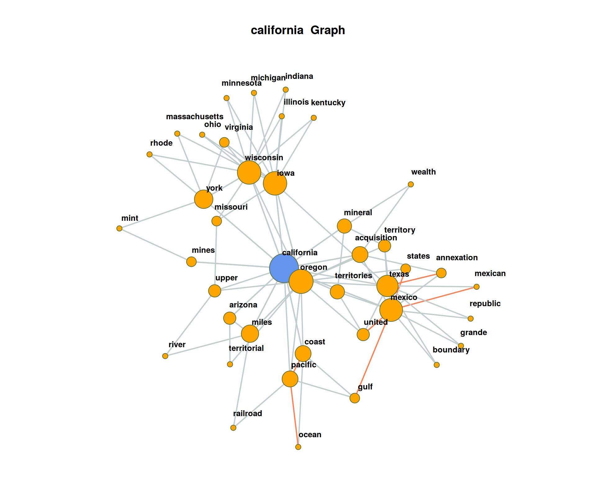
## 10  77.98097

4 Visualization of co-occurrence

In the following, we create a network visualization of significant co-occurrences.

For this, we provide the calculation of the co-occurrence significance measures, which we have just introduced, as single function in the file calculateCoocStatistics.R. This function can be imported into the current R-Session with the source command.

# Read in the source code for the co-occurrence calculation
source("calculateCoocStatistics.R")
# Definition of a parameter for the representation of the co-occurrences of a concept
numberOfCoocs <- 15
# Determination of the term of which co-competitors are to be measured.
coocTerm <- "california"

We use the imported function calculateCoocStatistics to calculate the co-occurrences for the target term “california”.

coocs <- calculateCoocStatistics(coocTerm, binDTM, measure="LOGLIK")

## Loading required package: slam

# Display the numberOfCoocs main terms
print(coocs[1:numberOfCoocs])

##      oregon      mexico       coast       upper     mineral       texas 
##   262.43281   114.40450    64.35717    52.87705    52.84182    51.69327 
## acquisition     pacific territories        york   wisconsin     arizona 
##    43.99069    40.75336    39.47065    36.87249    34.30973    33.98671 
##       mines        iowa       miles 
##    33.75958    29.69230    29.15576

To acquire an extended semantic environment of the target term, ‘secondary co-occurrence’ terms can be computed for each co-occurrence term of the target term. This results in a graph that can be visualized with special layout algorithms (e.g. Force Directed Graph).

Network graphs can be evaluated and visualized in R with the igraph-package. Any graph object can be created from a three-column data-frame. Each row in that data-frame is a triple. Each triple encodes an edge-information of two nodes (source, sink) and an edge-weight value.

For a term co-occurrence network, each triple consists of the target word, a co-occurring word and the significance of their joint occurrence. We denote the values with from, to, sig.

resultGraph <- data.frame(from = character(), to = character(), sig = numeric(0))

The process of gathering the network for the target term runs in two steps. First, we obtain all significant co-occurrence terms for the target term. Second, we obtain all co-occurrences of the co-occurrence terms from step one.

Intermediate results for each term are stored as temporary triples named tmpGraph. With the rbind command (“row bind”, used for concatenation of data-frames) all tmpGraph are appended to the complete network object stored in resultGraph.

# The structure of the temporary graph object is equal to that of the resultGraph
tmpGraph <- data.frame(from = character(), to = character(), sig = numeric(0))

# Fill the data.frame to produce the correct number of lines
tmpGraph[1:numberOfCoocs, 3] <- coocs[1:numberOfCoocs]
# Entry of the search word into the first column in all lines
tmpGraph[, 1] <- coocTerm
# Entry of the co-occurrences into the second column of the respective line
tmpGraph[, 2] <- names(coocs)[1:numberOfCoocs]
# Set the significances
tmpGraph[, 3] <- coocs[1:numberOfCoocs]

# Attach the triples to resultGraph
resultGraph <- rbind(resultGraph, tmpGraph)

# Iteration over the most significant numberOfCoocs co-occurrences of the search term
for (i in 1:numberOfCoocs){
  
  # Calling up the co-occurrence calculation for term i from the search words co-occurrences
  newCoocTerm <- names(coocs)[i]
  coocs2 <- calculateCoocStatistics(newCoocTerm, binDTM, measure="LOGLIK")
  
  #print the co-occurrences
  coocs2[1:10]
  
  # Structure of the temporary graph object
  tmpGraph <- data.frame(from = character(), to = character(), sig = numeric(0))
  tmpGraph[1:numberOfCoocs, 3] <- coocs2[1:numberOfCoocs]
  tmpGraph[, 1] <- newCoocTerm
  tmpGraph[, 2] <- names(coocs2)[1:numberOfCoocs]
  tmpGraph[, 3] <- coocs2[1:numberOfCoocs]
  
  #Append the result to the result graph
  resultGraph <- rbind(resultGraph, tmpGraph[2:length(tmpGraph[, 1]), ])
}

As a result, resultGraph now contains all numberOfCoocs * numberOfCoocs edges of a term co-occurrence network.

# Sample of some examples from resultGraph
resultGraph[sample(nrow(resultGraph), 6), ]

##         from       to      sig
## 1012 arizona  pursuit 12.27342
## 93     coast  eastern 79.07697
## 138  pacific    japan 79.06188
## 1014    iowa kentucky 31.11145
## 613    mines products 35.44232
## 1312 arizona governor 10.21321

The package iGraph offers multiple graph visualizations for graph objects. Graph objects can be created from triple lists, such as those we just generated. In the next step we load the package iGraph and create a visualization of all nodes and edges from the object resultGraph.

require(igraph)

# Set the graph and type. In this case, "F" means "Force Directed"
graphNetwork <- graph.data.frame(resultGraph, directed = F)

# Identification of all nodes with less than 2 edges
graphVs <- V(graphNetwork)[degree(graphNetwork) < 2]
# These edges are removed from the graph
graphNetwork <- delete.vertices(graphNetwork, graphVs) 

# Assign colors to edges and nodes (searchterm blue, rest orange)
V(graphNetwork)$color <- ifelse(V(graphNetwork)$name == coocTerm, 'cornflowerblue', 'orange') 

# Edges with a significance of at least 50% of the maximum sig- nificance in the graph are drawn in orange
halfMaxSig <- max(E(graphNetwork)$sig) * 0.5
E(graphNetwork)$color <- ifelse(E(graphNetwork)$sig > halfMaxSig, "coral", "azure3")

# Disable edges with radius
E(graphNetwork)$curved <- 0 
# Size the nodes by their degree of networking
V(graphNetwork)$size <- log(degree(graphNetwork)) * 5

# All nodes must be assigned a standard minimum-size
V(graphNetwork)$size[V(graphNetwork)$size < 5] <- 3 

# edge thickness
E(graphNetwork)$width <- 2

# Define the frame and spacing for the plot
par(mai=c(0,0,1,0)) 

# Finaler Plot
plot(graphNetwork,              
     layout = layout.fruchterman.reingold,  # Force Directed Layout 
     main = paste(coocTerm, ' Graph'),
     vertex.label.family = "sans",
     vertex.label.cex = 0.8,
     vertex.shape = "circle",
     vertex.label.dist = 0.5,           # Labels of the nodes moved slightly
     vertex.frame.color = 'darkolivegreen',
     vertex.label.color = 'black',      # Color of node names
     vertex.label.font = 2,         # Font of node names
     vertex.label = V(graphNetwork)$name,       # node names
     vertex.label.cex = 1 # font size of node names 
)

5 Optional exercises

1. Create term networks for “civil”, “germany”, “tax”

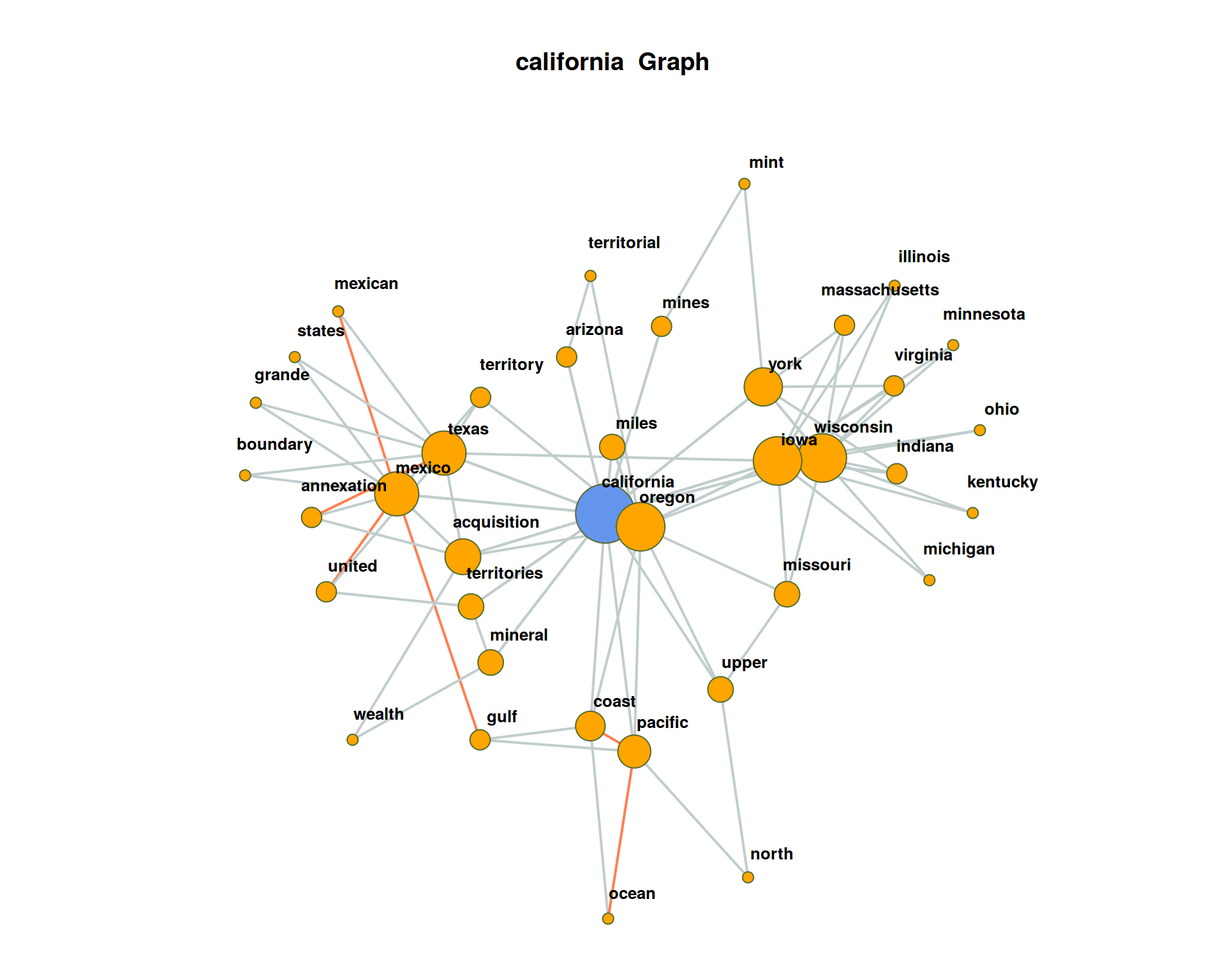
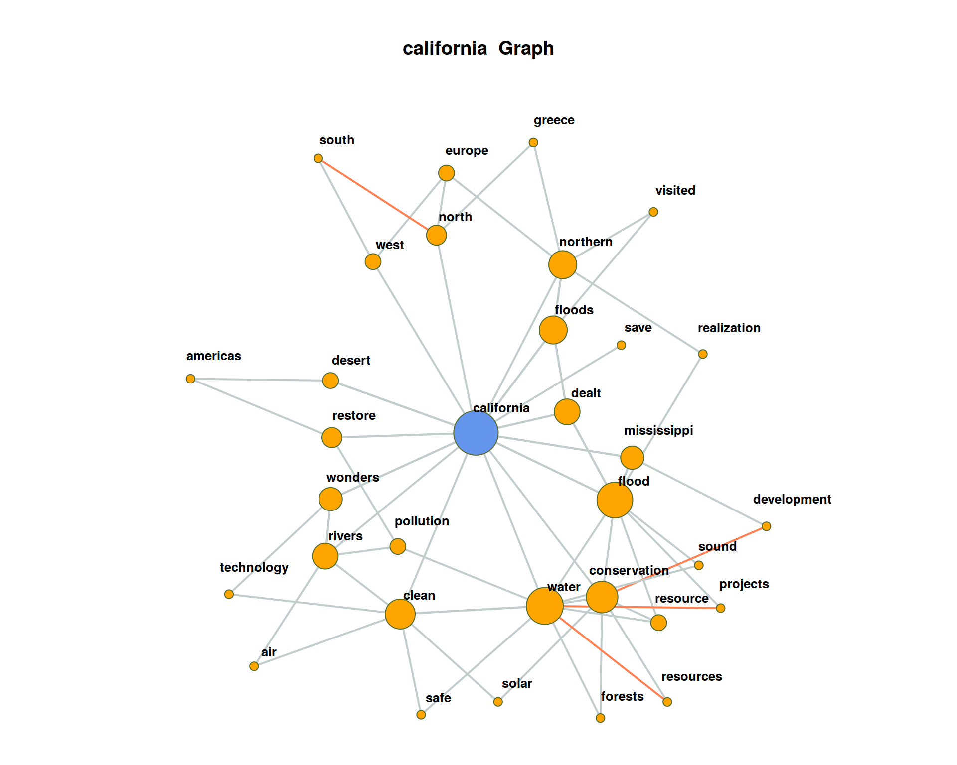
2. For visualization, at one point we filter for all nodes with less than 2 edges. By this, the network plot gets less dense, but we loose also a lot of co-occurring terms connected only to one term. Re-draw the network without this filtering. 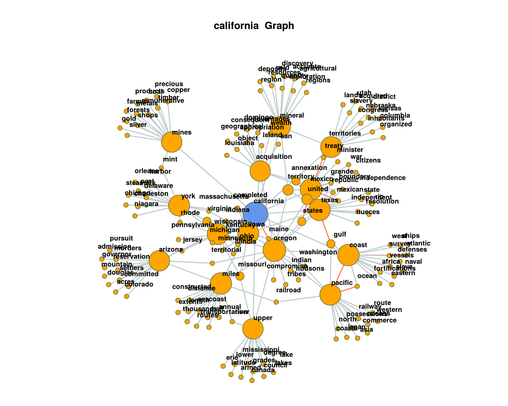The plot may get very messy. Try lower values for numberOfCoocs to create a less dense network plot.

3. Separate the DTM into two time periods (year < 1950; year > = 1950). Represent the graphs for the term “california” for both time periods. Hint: Define functions for the sub processes of creating a binary DTM from a corpus object (get_binDTM <- function(mycorpus)) and for visualizing a co-occurrence network (vis_cooc_network <- function(binDTM, coocTerm)).

## ===========================================================================

## ===========================================================================