1 Reading text data

Set global options at the beginning.

# Global options
options(stringsAsFactors = FALSE)

The read.csv command reads a CSV (Comma Separated Value) file from disk. Such files represent a table whose rows are represented by single lines in the files and columns are marked by a separator character within lines. Arguments of the command can be set to specify whether the CSV file contains a line with column names (header = TRUE orFALSE) and the character set.

We read a CSV containing 231 “State of the Union” addresses of the presidents of the United States. The texts are freely available from http://stateoftheunion.onetwothree.net. Our CSV file has the format: "id";"speech_type";"president";"date";"text". Text is encapsualted into quotes ("). Since sepration is marked by ; instead of ,, we need to specify the separator char.

# read csv into a data.frame
textdata <- read.csv("data/sotu.csv", header = TRUE, sep = ";", encoding = "UTF-8")

The texts are now available in a data frame together with some metadata (ID, speech type, president). Let us first see how many documents and metadata we have read.

# dimensions of the data frame
dim(textdata)

## [1] 231   5

# column names of text and metadata
colnames(textdata)

## [1] "id"          "speech_type" "president"   "date"        "text"

How many speeches do we have per president? This can easily be counted with the command table, which can be used to create a cross table of different values. If we apply it to a column, e.g. president of our data frame, we get the counts of the unique president values.

table(textdata[, "president"])

## 
##       Abraham Lincoln        Andrew Jackson        Andrew Johnson 
##                     4                     8                     4 
##          Barack Obama     Benjamin Harrison       Calvin Coolidge 
##                     8                     4                     6 
##     Chester A. Arthur       Donald J. Trump  Dwight D. Eisenhower 
##                     4                     1                     9 
## Franklin D. Roosevelt       Franklin Pierce      George H.W. Bush 
##                    12                     4                     4

Now we want to transfer the loaded text source into a corpus object of the tm-package. First we load the package.

require(tm)

Then, we crate with readTabular a mapping between column names in the data frame and placeholders in the tm corpus object. A corpus object is created with the Corpus command. As parameter, the command gets the data source wrapped by a specific reader function (DataframeSource, other reader functions are available, e.g. for simple vectors). The reader control parameter takes the previously defined mapping of metadata as input.

m <- list(ID = "id", content = "text")
myReader <- readTabular(mapping = m)
corpus <- Corpus(DataframeSource(textdata), readerControl = list(reader = myReader))
# have a look on the new corpus object
corpus

## <<VCorpus>>
## Metadata:  corpus specific: 0, document level (indexed): 0
## Content:  documents: 231

A corpus is an extension of R list objects. With the [[]] brackets, we can access single list elements, here documents, within a corpus.

# accessing a single document object
corpus[[1]]
# getting its text content
as.character(corpus[[1]])

## <<PlainTextDocument>>
## Metadata:  3
## Content:  chars: 6687

## [1] "Fellow-Citizens of the Senate and House of Representatives:\n\nI embrace with great satisfaction the opportunity which now..."

Success!!! We now have 231 speeches for further analysis available in a convenient tm corpus object!

2 Text statistics

A further aim of this exercise is to learn about statistical characteristics of text data. At the moment, our texts are represented as long character strings wrapped in document objects of a corpus. To analyze which word forms the texts contain, they must be tokenized. This means that all the words in the texts need to be identified and separated. Only in this way is it possible to count the frequency of individual word forms. A word form is also called “type”. The occurrence of a type in a text is a “token”.

For text mining, text are further transformed into a numeric representation. The basic idea is that the texts can be represented as statistics about the contained words (or other content fragments such as sequences of two words). The list of every distinct word form in the entire corpsu forms the vocabulary of a corpus. For each document, we can count how often each word of the vocabulary occurs in it. By this, we get a term frequency vector for each document. The dimensionality of this term vector corresponds to the size of the vocabulary. Hence, the word vectors have the same form for each document in a corpus. Consequently, multiple term vectors representing different documents can be combined into a matrix. This data structure is called document-term matrix (DTM).

The function DocumentTermMatrix of the tm package creates such a DTM. If this command is called without further parameters, the individual word forms are identified by using the “space” as the word separator.

# Create a DTM (may take a while)
DTM <- DocumentTermMatrix(corpus)
# Show some information
DTM

## <<DocumentTermMatrix (documents: 231, terms: 54333)>>
## Non-/sparse entries: 466743/12084180
## Sparsity           : 96%
## Maximal term length: 35
## Weighting          : term frequency (tf)

# Dimensionality of the DTM
dim(DTM)

## [1]   231 54333

The dimensions of the DTM, 231 rows and 54333 columns, match the number of documents in the corpus and the number of different word forms (types) of the vocabulary.

A first impression of text statistics we can get from a word list. Such a word list represents the frequency counts of all words in all documents. We can get that information easily from the DTM by summing all of its column vectors.

A so-called sparse matrix data structure is used for the document term matrix in the tm package (tm imports the slam package for sparse matrices). Since most entries in a document term vector are 0, it would be very inefficient to actually store all these values. A sparse data structure instead stores only those values of a vector/matrix different from zero. The slam package provides arithmetic operations on sparse DTMs.

require(slam)

## Loading required package: slam

# sum columns for word counts
freqs <- col_sums(DTM)
# get vocabulary vector
words <- colnames(DTM)
# combine words and their frequencies in a data frame
wordlist <- data.frame(words, freqs)
# re-order the wordlist by decreasing frequency
wordIndexes <- order(wordlist[, "freqs"], decreasing = TRUE)
wordlist <- wordlist[wordIndexes, ]
# show the most frequent words
head(wordlist, 25)

##                 words  freqs
## the               the 150070
## and               and  60351
## that             that  21328
## for               for  18916
## our               our  17438
## with             with  11967
## have             have  11941
## which           which  11900
## this             this  11845
## will             will   9245
## has               has   8962
## are               are   8804
## not               not   8708
## been             been   8695
## their           their   7788
## from             from   7467
## all               all   6355
## its               its   5755
## was               was   5599
## but               but   5536
## government government   5163
## should         should   5076
## they             they   4945
## united         united   4798
## states         states   4480

The words in this sorted list have a ranking depending on the position in this list. If the word ranks are plotted on the x axis and all frequencies on the y axis, then the Zipf distribution is obtained. This is a typical property of language data and its distribution is similar for all languages.

plot(wordlist$freqs , type = "l", lwd=2, main = "Rank frequency Plot", xlab="Rank", ylab ="Frequency")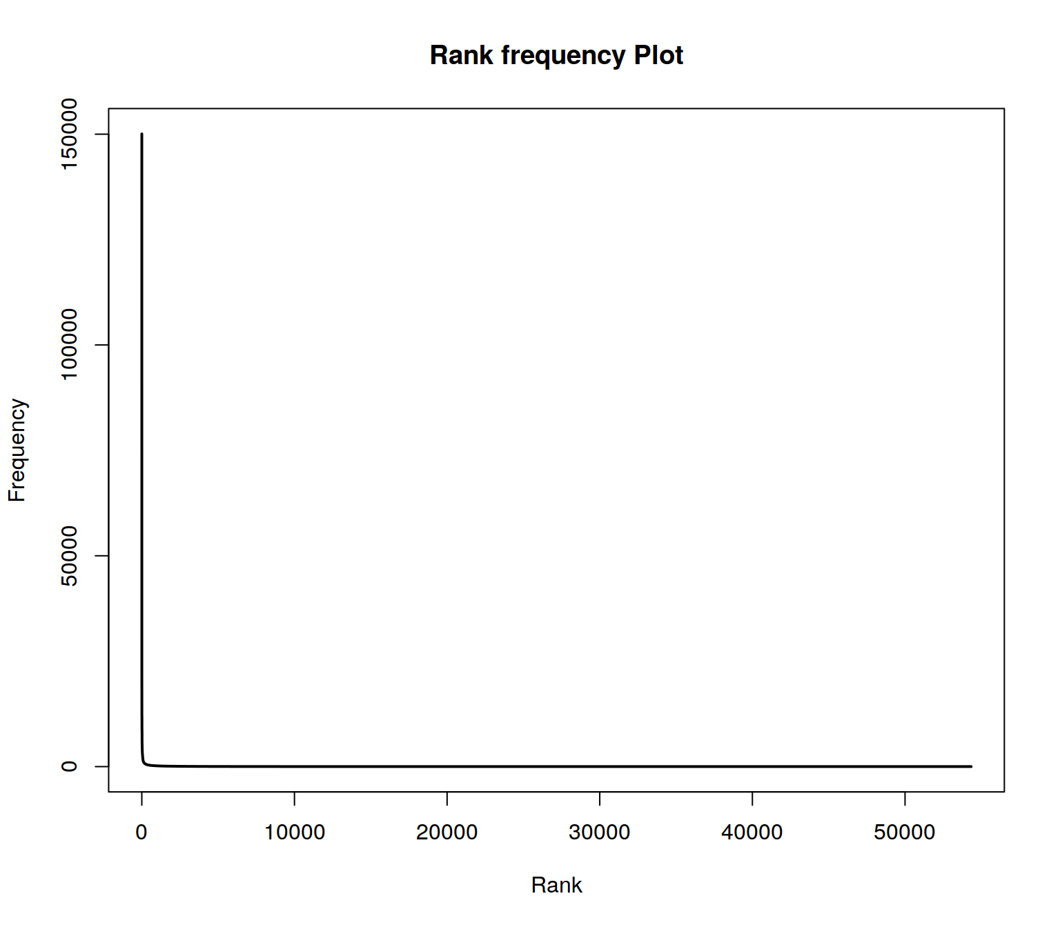

The distribution follows an extreme power law distribution (very few words occur very often, very many words occur very rare). The Zipf law says that the frequency of a word is reciprocal to its rank (1 / r). To make the plot more readable, the axes can be logarithmized.

plot(wordlist$freqs , type = "l", log="xy", lwd=2, main = "Rank-Frequency Plot", xlab="log-Rank", ylab ="log-Frequency")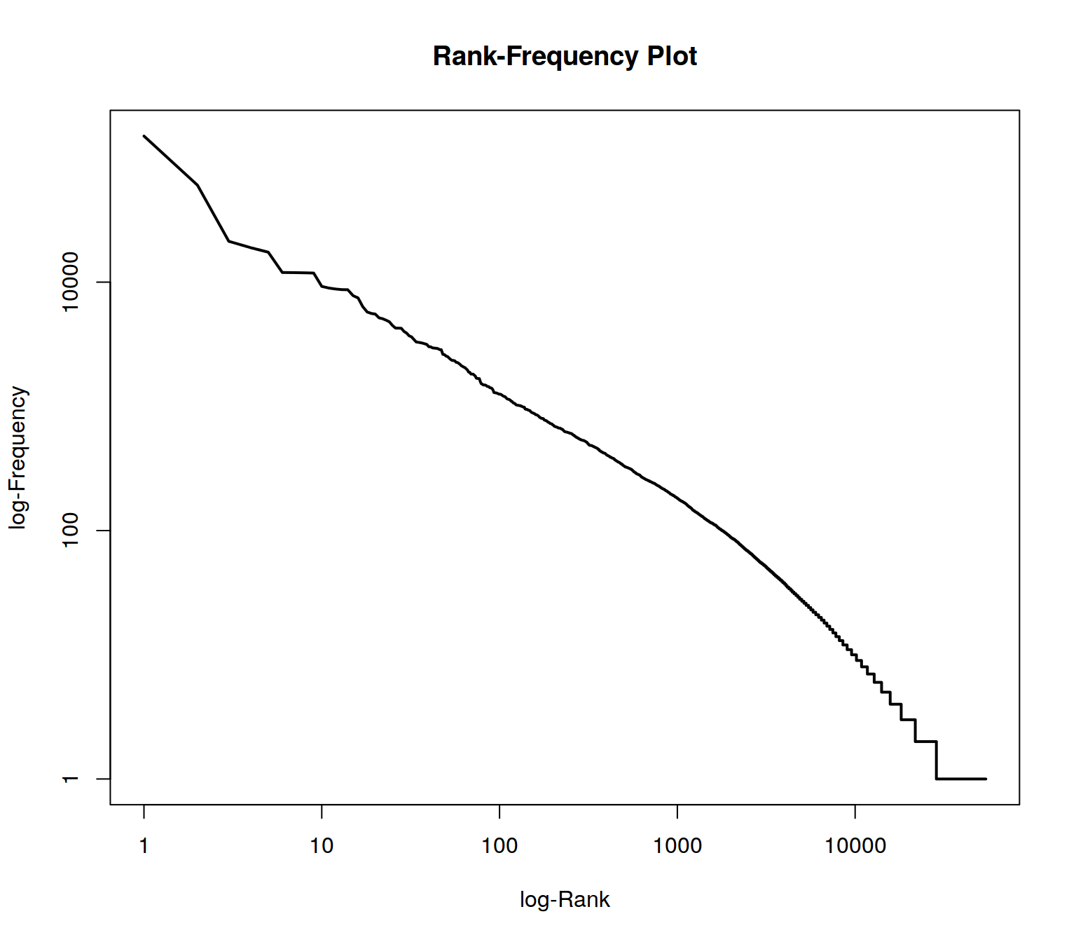

In the plot, two extreme ranges can be determined. Words in ranks between ca. 10,000 and 54333 can be observed only 10 times or less. Words below rank 100 can be oberved more than 1000 times in the documents. The goal of text mining is to automatically find structures in documents. Both mentioned extreme ranges of the vocabulary often are not suitable for this. Words which occur rarely, on very few documents, and words which occur extremely often, in almost every document, do not contribute much to the meaning of a text.

Hence, ignoring very rare / frequent words has many advantages:

• reducing the dimensionality of the vocabulary (saves memory)
• processing speed up
• better identification of meaningful structures.

To illustrate the range of ranks best to be used for analysis, we augment information in the rank frequency plot. First, we mark so-called stop words. These are words of a language that normally do not contribute to semantic information about a text. In addition, all words in the word list are identified which occur less than 10 times.

The %in% operator can be used to compare which elements of the first vector are contained in the second vector. At this point, we compare the words in the word list with a loaded stopword list (retrieved by the function stopwords of the tm package) . The result of the %in% operator is a boolean vector which contains TRUE or FALSE values.

A boolean value (or a vector of boolean values) can be inverted with the ! operator (TRUE gets FALSE and vice versa). The which command returns the indices of entries in a boolean vector which contain the value TRUE.

We also compute indices of words, which occur less than 10 times. With a union set operation, we combine both index lists. With a setdiff operation, we reduce a vector of all indices (the sequence 1:nrow(wordlist)) by removing the stopword indices and the low freuent word indices.

With the command “lines” the range of the remining indices can be drawn into the plot.

plot(wordlist$freqs, type = "l", log="xy",lwd=2, main = "Rank-Frequency plot", xlab="Rank", ylab = "Frequency")
englishStopwords <- stopwords("en")
stopwords_idx <- which(wordlist$words %in% englishStopwords)
low_frequent_idx <- which(wordlist$freqs < 10)
insignificant_idx <- union(stopwords_idx, low_frequent_idx)
meaningful_range_idx <- setdiff(1:nrow(wordlist), insignificant_idx)
lines(meaningful_range_idx, wordlist$freqs[meaningful_range_idx], col = "green", lwd=2, type="p", pch=20)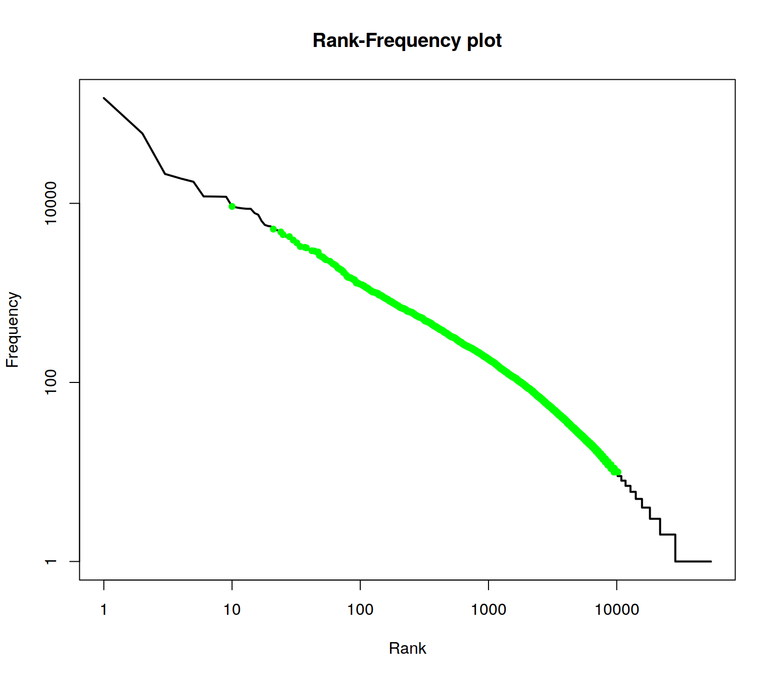

The green range marks the range of meaningful terms for the collection.

3 Optional exercises

1. Print out the word list without stop words and low frequent words.

##                 words freqs
## will             will  9245
## government government  5163
## united         united  4798
## states         states  4480
## can               can  4255
## upon             upon  3893
## congress     congress  3626
## may               may  3299
## must             must  3227
## great           great  3189
## public         public  2957
## new               new  2934
## people         people  2865
## made             made  2860
## now               now  2622
## american     american  2543
## one               one  2519
## year             year  2451
## time             time  2391
## last             last  2347
## every           every  2255
## national     national  2123
## country       country  2069
## present       present  2003
## war               war  1887

2. If you look at the result, are there any corpus specific terms that should also be considered as stop word?
3. What is the share of terms regarding the entire vocabulary which occurr only once in the corpus?

## [1] 0.4728986

4. Compute the type-token ratio (TTR) of the corpus. the TTR is the fraction of the number of tokens divided by the number of types.

## [1] 0.03876839